
It’s no surprise that lots of landlords use spreadsheets to manage their properties. When you first start out, maybe you’ve got one or two rental properties and only a handful of tenants, in which case your spreadsheet is enough.
If you’re new to the world of spreadsheets, or you’ve never delved into the confusingly named Excel features it’s easy to get lost in the whirlpool of Excel functions and formulas.
In this article I’m going to take you through 7 Excel tips – in detail, with screenshots – that landlords need to know. If you’re an Excel master these may not be new to you, but a knowledge refresh never hurt anyone.
Before we get down to the details, I want to let you know that we offer a free spreadsheet you can download that’s been created specifically for landlords to manage their income and expenditure. So, if all this talk of Excel is already giving you jitters, skip the technical mumbo jumbo and get straight to the numbers by downloading your free landlord income and expense spreadsheet.
Onwards to the Excel functions…
Here’s what we’ll be covering. Skip to the bit that interests you by clicking the orange links in the list below, or read (and bookmark) the whole thing for future reference:
- Spreadsheet Formatting – No one likes a messy or broken spreadsheet, this is how you fix it
- Paste Options – More exciting than it sounds, let me take you beyond copy and paste
- Conditional Formatting – Make important cells and information stand out automatically
- Spelling and Grammar – Because it’s not switched on as standard in Excel
- Wrap Text – It’s nice to be able to read things without having huge columns
- Data Filter – Find what you need quickly by filtering the information in your columns
- Formula Auditing – Giving you the information that #Name! and #DIV/0! won’t
- Bonus Tip – Stylistic suggestions for professional looking spreadsheets
Format Like a … Formatter? – How to format your landlord spreadsheet
No one likes a messy spreadsheet. Have you ever copied and pasted something into a spreadsheet only to find out that the text is somehow bigger, or a different colour, or it mucks about with your borders?
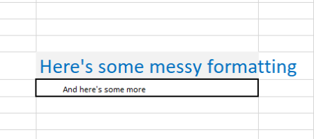
You then spend ages trying to find all the formatting options to make it look like every other cell in your spreadsheet! Well, there’s a tool for that.
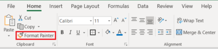
The format painter does what it says on the tin, it copies a format you choose from an existing cell and applies it to another one. Here’s where you’ll find it:
The instructions given in Excel are straightforward:
- Select content with the formatting you like
- Click format painter
- Select something else to automatically apply the formatting
The format painter won’t copy formulas or text, just formats like font, size, cell colour and borders.
Another little-known format painter trick is to click format painter twice, this means it will continue to apply the copied format to any cell you click until you click format painter again to turn it off – that’s really useful if you have a lot of squiffy formatting.
(Bonus tip – the format painter is available in most Microsoft programmes including Outlook and Word).
Copy and Paste like a Pro
This goes hand in hand with the tip above. While it’s easy to adjust the formatting with format painter, you may be able to avoid all that in the first place by using the right paste options in Excel. We’re about to go way beyond copy and paste.
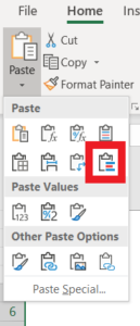
If you are copying and pasting from anything other than a spreadsheet and you click the little down arrow underneath the paste button in the main menu you’ll be given three options:
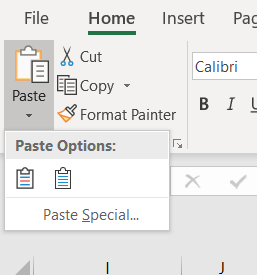
If you hover over the paste option icons you’ll be given a short description of each one:
-
- Keep source formatting (meaning don’t change how the formatting looks when I paste it in)
- Match destination formatting (meaning make the formatting look like the formatting in the rest of the spreadsheet when I paste it in)
- Paste special, which even I don’t understand!
The two formatting options are a great way to avoid ending up with a Frankenstein’s monster of a spreadsheet when copying and pasting.
If you copy and paste from a spreadsheet to a spreadsheet there’s a whole new world of useful paste options that are mostly self-explanatory.
Click the little arrow under the paste button. If you hover over an icon, Excel will tell you which paste function it relates to.
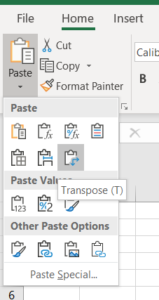
Here’s a cursory simplified look at all the available paste options in Excel and what they mean:
-
- Paste – Just a straightforward copy and paste.
- Formulas – Pastes only the formulas.
- Formulas and number formatting – Pastes the formulas and the number formatting (number formatting is things like percentages, decimal places etc).
- Keep source formatting – Won’t change the format of the data you are pasting in.
- No borders – Pastes information without borders (useful if you’re copying numbers from a table with borders and you don’t want to keep the border outlines).
- Keep source column widths – Paste the data using the same column width as the column it came from.
- Transpose – If you have data in a vertical list and you select this option it will paste it as a horizontal list and vice versa.
- Values – This will paste only the numbers in the cells and ignore any formulas.
- Values and number formatting – Pastes the numbers and the number formatting (like percentages) but will ignore formulas.
- Values and source formatting – This will paste the numbers, ignore formulas and won’t make any changes to the formatting.
- Formatting – Paste just the formatting and none of the data (like format painter but works across different documents).
- Paste link – Paste the data as a link – this will paste all the data you’ve copied, but it will remain linked to the source. This is a useful way to make multiple spreadsheets work together. Data that’s pasted in this way updates automatically when the place you pasted the data from is updated. This is really useful for creating a dashboard for instance but can get quite messy if you’re linking lots of different spreadsheets.
- Picture – Paste the data you’ve copied as a picture.
- Linked picture – This works in a similar way to paste link. It can paste any excel selected data as a picture, the picture automatically updates when the source data is updated. Another useful one for creating dashboards using pictures.
Conditional Formatting for eagle-eyed landlords
Back in the bad old days you had to know and understand how to write rules for conditional formatting, it was as painful as learning algebra but at least it was more satisfying when you finally worked it out. These days Microsoft has made things a little easier with automated rules.
Conditional formatting allows you to apply a format to a cell if certain rules are met. How does that help you as a landlord? Well what if you could make a cell red if your tenant is behind on payments? Or what if you had a list of dates for tenancy renewals and you could make them orange if they’re due soon? These things are possible with conditional formatting.
It’s still possible to write your own custom rules, but if you aren’t an expert, Microsoft’s auto rules are versatile and can be found on the home tab:

First up we’ll take a look at the highlight cells rules, these allow you to say to your spreadsheet: ‘hey, if one of my cells says x, make it look different so I can spot it easily.’
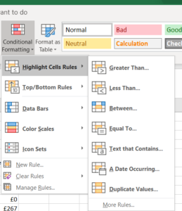
In the screenshot above you can see the different types of rules you can apply, for instance highlight cells that are greater than a number you specify. When you click on one of these options you get the chance to refine the rules.
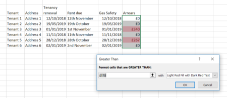
In this example you can see I’ve clicked on highlight cells that are greater than, this dialogue box then allows me to specify the number that triggers the formatting. On the right hand side of the dialogue box you can see it will make the cell red with dark red text if the number is greater than the one I’ve specified. You can change this format to anything you like using the downward arrow.
Each of the conditional formatting rules for highlight cells and top and bottom values are quite well explained with the dialogue boxes that pop up. When you look at data bars, colour scales and icon sets it’s a little less intuitive.
Essentially data bars show a bar inside the cell, its length depends on how high the number in the cell is.
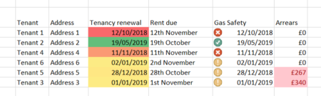
Colour scales are a lot simpler. They allow you to apply a colour gradient to a set of data that gives it a red amber green status. Let me demonstrate using the tenancy renewal column in my spreadsheet:
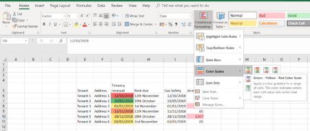
This is a nice easy time saving trick that replaces the need to add in lots of highlight cell rules. I didn’t have to enter any additional data. Excel has used the data I highlighted to figure out a red, amber, green, scheme. The red dates are overdue, and the green dates are far away, anything in the middle is due soon. Excel has based this scale on the extremes of the data I’ve selected. It recognises we’re working with dates and so it has determined the closest date and the one furthest away and built the scale based on that information.
If you were to apply the colour scale to a list of numbers the colour scale would be worked out based on the highest and lowest numbers. Using the colour scale in the screenshot above would mean that higher numbers were green and lower numbers were red. You may want to reverse this for something like rental arrears where you’d like high numbers to be red instead of green. You can change this by looking at the direction of the gradient on the colour scale you are using. In the screenshot above you’ll notice the first gradient is green to red (the one that’s selected) the second gradient is red to green, this will reverse the formatting rules to highlight lower numbers green.
The icon sets conditional formatting will add icons to your cells, they work similarly to the colour scales rules, you can highlight some cells, click on icon sets, choose your set and Excel will work out what each symbol should represent. Symbols are things like arrows to show where numbers are up or down, red, amber, green flags and a whole host of bits and pieces that would work well for project management.
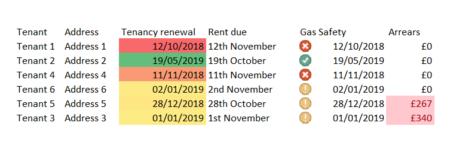
I’ll show you an example using my Gas Safety column:
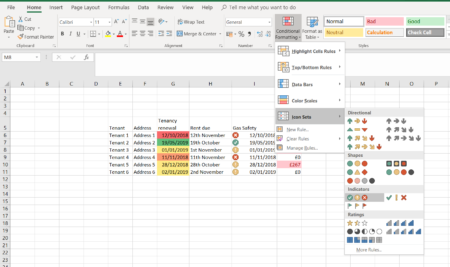
So here I’ve applied the tick, cross and exclamation indicators to my Gas Safety column. The crosses show that some of the gas safety certs are overdue or are due within a month, exclamation marks show they’re more than a month away but due soon, and a tick shows the due date is far in the future.
Hopefully you can see how this is useful for landlords, it makes it easier to spot the important information in your spreadsheet quickly.
Another quick tip that might save you a few handfuls of hair down the line: if you want to edit or delete your conditional formatting, select the cells you want to edit and go to ‘conditional formatting’ manage rules. Here you can also tweak the rules associated with your icon sets and colour scales.
Once you’ve got conditional formatting in your spreadsheet, you’ll get a new paste option in Excel called merge conditional formatting:
This will allow you to copy and paste any conditional formatting rules along with your data.
Spelling and Grammar for Presentable Property Owners
This next one is a simple tip, but it took me ages to work out, so I’ll share it here. In Excel, spelling and grammar is not switched on as standard. Your spelling and grammar errors will only show up if you manually start a spelling and Grammar check. This is good to know if good spelling and grammar is important to you, or if you want to share your spreadsheet with someone else.
You’ll find the spell check button (and a thesaurus should you ever need it) in the review tab.
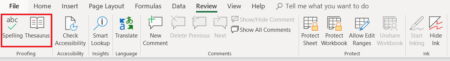
Just remember, if you’ve selected a group of cells with your mouse before clicking this button, the spellcheck will only check what’s in the selected cells.
Wrap Text – Not warp text, just a better way to organise your landlord spreadsheets
I once made a lot of people laugh when I referred to this as a word warp, word wrap makes much more sense! Another simple tip but one that I use all the time. If you don’t want to adjust your column width to accommodate lengthy text like addresses, you can use wrap text. This allows the cell to extend vertically to automatically encompass your text.
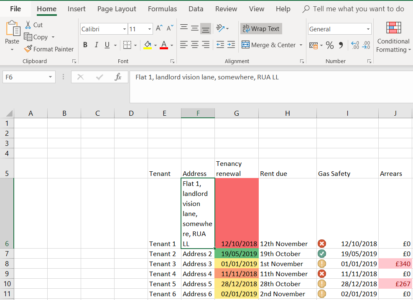
Bonus tip, if you’ve used wrap text, the cell will automatically adjust if you edit the data. It will also stretch the other cells in the row as you can see from the screenshot above.
Data Filter – Find what matters to you quickly
Do not be afraid of the data filter, this is more useful the larger your spreadsheets get. If you have named your columns well, and all the headings line up in one row, you can filter the data in the columns.
I’ll show you using my spreadsheet. Select all the headings you want to filter, click into the data menu tab, then click filter:
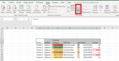
This has now added little drop down arrows next to my headings that I can use to filter the data in each column, so If I wanted to filter by arrears I can click the arrow next to arrears and filter by the data in that column:
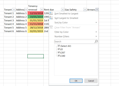
You can also filter by colour, text and number. Just be aware that if you use the sort options at the top of this dialogue box, there’s no easy way to remove them. Filters on the other hand can be cleared by using the ‘clear filter’ button.
You can remove the data filter from your spreadsheet at any point by just clicking the filter button again. This will remove any applied filters, but if you’ve used sort, the data will remain sorted even after you remove the data filter.
Formula Auditing – For landlords who like spreadsheet formulas
It’s so frustrating when you’re putting formulas together and they don’t work. All you get is a notification in your cell such as: #Name! or #DIV/0! often the information Microsoft gives you as to why the formula is broken may as well be written in Greek. Helpfully though, Excel has some formula auditing tools, these are a great way of finding out why your formula isn’t working.
Trace Precedents
If you click this button Excel will use arrows to show you formulas or data that contribute to the formula in the cell you’re auditing.
So if your formula is the value of three other cells added together, those three other cells are your Precedents, if you click the trace precedents button, Excel will demonstrate that for you:
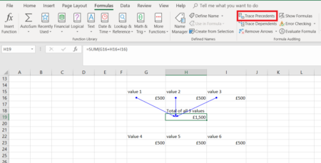
This is useful for checking that the information going into your formula is correct.
Trace Dependents
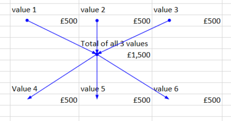
This will also use arrows to show you any formulas or values that are dependent on the formula you are auditing. Back to the spreadsheet example:
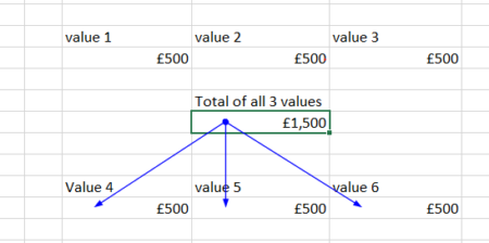
The green box in the screenshot is where the formula is. The formula has determined that £1,500 is the total of values 1-3. To work out values 4-6 I’ve written a formula that divides the result of the formula in the green box by 3. Values 4-6 rely on the formula in the green box so they are dependents.
If you click both precedents and dependents you’ll get both sets of arrows at once:
A little counter-intuitively, when you use trace precedents and dependents, the only way to remove the arrows that Excel gives you is to click remove arrows in the menu:
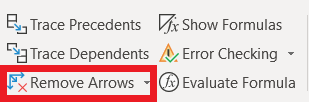
This little gem of information would have saved me over an hour the first time I used this function!
Show Formulas
Does just that, instead of showing the error or the value of the formula, the formula will appear in the cell, this can be a bit easier for editing purposes, especially if you’re working with long formulas. To make the formulas disappear again, click the show formulas button again.
Here’s the same spreadsheet I used to show trace precedents and descendants with all the formulas shown:
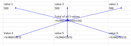
As you can see, using the formulas and the tracing tools at the same time can highlight the logic behind your formulas.
Error Checking
Works just like spell check but for formulas. Once you’ve built your sheet click this button and any errors will be highlighted. This is really only useful if you have loads and loads of formulas as Excel will generally show you in the cell if there’s an error.
Here’s an example where Excel has picked up an incomplete formula:
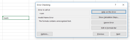
You’ll get a few options in this dialogue box that will help you correct the mistake.
Evaluate Formula
This allows you to work through a formula step by step, the dialogue box shows you how Excel interprets and acts on the formula allowing you to find out which part of it isn’t working. This is a great tool if you’re using long decision making formulas like IF, IFS, AND, COUNTIFS etc.
Here’s an example of the dialogue box:
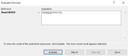
Here it shows you the formula it’s evaluating, the underlined bit of the formula tells you the first calculation that Excel makes. If you click evaluate, it replaces the cell number with the actual value. Continue to evaluate and you’ll see step by step how Excel is running through your formula, which can help you find the unwanted bit really quickly.
Bonus Tip – Stylistic Suggestions for suave landlord spreadsheets
Sometimes you’ll need a spreadsheet to look professional. A lot of the tips in this guide will have your spreadsheet looking fancy in no time, but if you want to take it to the next level, here are some top tips for suave spreadsheets.
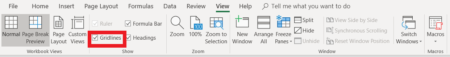
Every Excel spreadsheet has pale gridlines, these are there to make sorting and arranging data easier, but they aren’t to everyone’s liking. It’s possible to remove these gridlines from the whole sheet giving it a crisp fresh feel.
If you’re trying to make your spreadsheet look good or smart this is often a good place to start. Remove the gridlines from your sheet and instead use borders and colours to make your sheet look professional.
Before
After
To turn the gridlines on or off, click into the view tab and tick or un-tick the gridlines checkbox:
Once you’ve removed the gridlines, you can style your spreadsheet or group data using cell fill colour and borders, check out these examples created with cell fill and border styles:
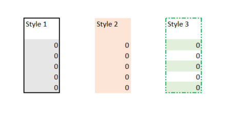
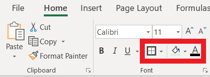
All the border and cell fill options can be found in the font section of the home menu:
Phew, I feel less like they were tips and more like a re-education in Excel! If you can think of any tips that would benefit your fellow landlords, drop them in the comments so we can all share the spreadsheet love. <3
Want the free landlord income and expenditure spreadsheet before you go?
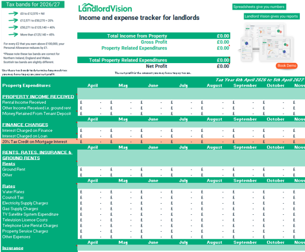
If you don’t fancy building an Excel spreadsheet of your own, you could start with our free income and expenses spreadsheet. This has been put together by landlords who have used spreadsheets to manage their own properties.
The spreadsheet has been updated for the current tax year, so all you need to do is pop your income and expenditure details in and everything will be worked out for you. (There’s even a handy tax bracket guide and the expenses section acts as a great reminder on deductible expenses).
Did we miss anything? Or have you got some great spreadsheet tips of your own? Share them in the comments.